

Pressure Vessel Engineering has been doing CFD and Thermal Analyses for a number of years when our customers have had a need for this type of service. In a few upcoming articles, we’ll explain how we use our software and demonstrate why it will be a valid solution for you that will save both time and cost on your projects.

Waste Heat Recovery Shell and Tube Heat Exchanger For Gas Turbine
Gas turbines are used in many applications including power generating stations, cogeneration plants, and in the oil and gas industry to provide power in remote offshore and onshore production facilities locations.

Exploring Thermal Efficiency in Electrical Heaters: A CFD Analysis
Thermal efficiency plays a crucial role in the performance of electrical heaters, impacting energy consumption, operational cost, and overall system effectiveness. This study aims to understand how changes in velocity, the presence of baffles and the orientation of the baffles affect heat transfer efficiency.

Optimizing Thermal Stratification in Chilled Water Thermal Energy Storage Tanks Using CFD
Gas turbines are used in many applications including power generating stations, cogeneration plants, and in the oil and gas industry to provide power in remote offshore and onshore production facilities locations.
Validation of SolidWorks Flow Simulation CFD software
Validation is a vital method for knowing the strengths and weaknesses of Computational Fluid Dynamics (CFD) software. Without it you will not know when the program is producing good results, or when it is producing results that need additional analysis before use. Three CFD validation sets follow: First, a flat plate heat transfer simulation produced final and accurate results very qucikly. Second, a pressure drop through a straight pipe study produced results that converged to an approximate finish point very slowly and could not reach an ultimate calculated value. Different methods are required for heat transfer and pressure drop.
Finally, the comparison of pressure drops in two 180° elbows shows a method to overcome the limitations of pressure drop convergence. The relative difference between two designs is studied instead of looking for absolute pressure drops which are never reached. As with the heat transfer study, useful results are obtained, but this time more work is involved.
Validation Example – Flat Plate Heat Transfer
Validation Example – Flat Plate Heat Transfer
File PVE-11617 – LRB, CBM – May 11 2017
Heat transfer between fluids and the pressurized equipment that contains it is of interest to our customers. We use SolidWorks Flow Simulation which can solve many flow problems including heat transfer. Flow Simulation ships with validation samples including #10 “Flow Over a Heated Plate”. SolidWorks compares their results against published data. Our interest is to learn how much computing resources are required to get a good result? Is it practical to use flow simulation to solve heat transfer problems?

SolidWorks Flow Simulation validation problem #10 “Flow Over a Heated Plate
Validation Example #10 is a simple 2D study of flow of air over a heated flat plate. 1 atmosphere air at 293.2 K (20 C) and inlet velocity of 1.5 m/s passes over a plate 0.31 m long. The plate is heated to maintain its temperature at 303.2 K, 10 K warmer than the inlet air temperature. The boundary layer starts at the leading edge of the heated plate. How does the heat transfer rate vary along the length of the plate?

The developed boundary layer for this problem. Fluid temperature is shown in solid colors, pressure drop by white isobars.
This is the results we got at mesh #5, the final mesh used in this study. The development of the boundary layer from zero thickness at the left end of the plate can be seen from the temperature plot. The pressure drop is also plotted with white isobars. The temperature profile makes sense.

Results obtained by SolidWorks. Case 1- the flow simulation results (blue line) closely match the published results (red line)
SolidWorks found a close match between the published results and the heat transfer rate calculated by Flow Simulation.
How much computer resources are required to get good results? We started with a very coarse initial mesh (mesh #1 below) and programmed Flow Simulation in a four step process:
- Solve the flow problem with the mesh given and save the results.
- Determine which cells have converged and which need refinement (non-converged)
- Divide each non-converged cell into 4 smaller identical cells.
- Do not change the cells that have converged. Repeat step #1 ten times.
This was run on a medium power computer: i7 6600U CPU @ 2.6-2.81 GHz (2 physical cores, 4 hyper threaded cores), 16 GB ram. Very little ram was used in the study.

Average heat transfer rate by iteration. “*” marks when the mesh was refined by dividing cells. At mesh 5 complete convergence is obtained and the mesh has finished refining.
Flow Simulation repeated the above four step process ten times. By mesh #5 all cells were converged. The remaining five iterations resulted in no new mesh, the process was complete. Total time 111 seconds.

Auto-generated meshes produced by this study
- Mesh #1 – All cells are identical in a 8×2 Gird (16 cells, iteration 45, 6 seconds). All cells are non-converged, all are divided into 4 identical cells to create mesh #2.
- Mesh #2 – All cells are identical, mesh size is 16×4 (64 cells, iteration 146, 16 seconds). Some cells at the top have reached convergence and will not be divided again, others near or at the heated plate need to be divided.
- Mesh #3 – First mesh with different cell sizes (576 cells, iteration 228, 26 seconds). The light blue cells have reached convergence and will not be divided more. Some green cells in the middle have also reached convergence. The cells next to the heated plate need to be further divided.
- Mesh #4 – The mesh now has 3 different cell sizes (2340 cells, iteration 311, 39 seconds). The blue, green and some yellow cells are fully converged and will not be further divided. Again some of the cells next to the heated plate will be divided.
- Mesh #5 – The final mesh (9396 cells, iteration 450, 90 seconds). All the cells have reached convergence. Although the program has five more iterations, no further cell division happens.

Heat transfer along plate vs mesh
How fast does the heat transfer rate converge? Although the program continued refining the mesh until mesh 5 (90 seconds), the results had practically converged by step 3 at 39 seconds. However the additional runs producing the same results proved that convergence had been reached. This is fast convergence. Flow simulation provided good results even with a coarse mesh. This makes it practical to use flow simulation on available computers to solve heat transfer problems.
Pressure Drop in a Straight Pipe
Pressure Drop in a Straight Pipe
PVE-11633 and 7479 / LRB and CBM /May 18 2017
Flow induced pressure drop in a straight pipe is well studied making it a good subject for validating the results from SolidWorks Flow Simulation (called Flow Simulation in this article) a Computational Fluid Dynamics (CFD) program.
The validation case is a straight pipe 0.01905 m (0.75″) inside diameter, 0.009525 m radius (0.375″) by 0.18796 m long (7.40″) has 293.2 K (20 C 68°F), water flowing through it at an average velocity of 1 m/s (3.281 ft/s). The pipe wall is assumed to be perfectly smooth. Inlet flow condition is assumed to be fully developed. The outlet static pressure is set to 101,325 Pa (1 atmosphere). Calculate the average pressure drop from inlet to outlet.

Figure 1: The straight pipe used for this validation case. The CFD is simplified to a quarter model using symmetry in two planes.
Theory
Straight pipe pressure drop calculators based on textbook methods are available . Here “Pressure Drop Online-Calculator” is used (http://www.pressure-drop.com/Online-Calculator/)
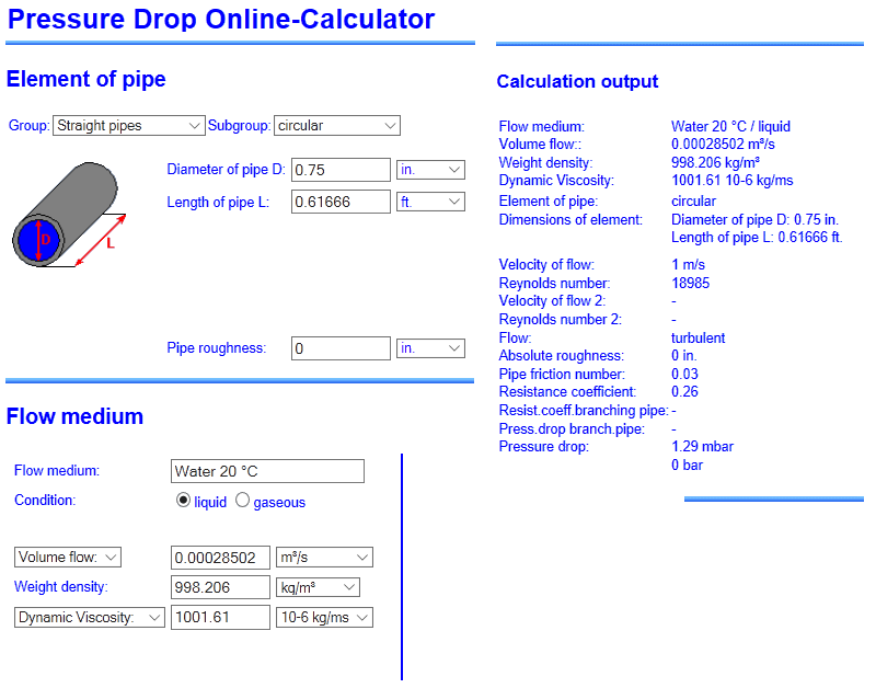
Figure 2: Using textbook methods, a pressure drop of 1.29 mbar or 129 Pa is predicted
The predicted pressure drop is 1.29 mbar or 129 Pa.
Flow Simulation
The validation case was modeled in SolidWorks and solved in Flow Simulation. Symmetry in both the XZ and YZ planes was used to reduce the mesh complexity by four. Initially a very coarse mesh was used. Our standard four step iterative mesh refinement process was programmed into Flow Simulation:
- Solve the 3D flow problem with the given mesh and save the results.
- Determine which cells have converged and which need refinement (non-converged)
- Divide each non-converged solid cell into 8 smaller cells.
- Do not divide the cells that have converged. Repeat step #1 ten times.
This was run on our most powerful computer: i7 6850U CPU @ 3.6 GHz (6 physical cores, 12 hyper threaded cores), 128 GB ram. Processing was stopped by the operator after 16 hours when mesh 7 reached convergence. The three remaining meshes were not run because all available computer resources had been used. A final converged result had not been reached.
Flow Simulation Results:
| Mesh | Iteration | Cells | Time | Drop (Pa) | Error | Comment |
|---|---|---|---|---|---|---|
| 1 | 53 | 576 | 2 s | 77.6 | -39.8% | One mesh size only – all cells need refining |
| 2 | 83 | 4,224 | 5 s | 118.5 | -8.1% | One mesh size only – all cells need refining |
| 3 | 131 | 30,822 | 22 s | 133.1 | 3.2% | Two mesh sizes – central channel cells do not need further refining |
| 4 | 220 | 176,759 | 3 min | 144.8 | 12.2% | Three mesh sizes – further separation of coarse and fine areas – |
| 5 | 347 | 662,364 | 20 min | 141.6 | 9.8% | Four mesh sizes – first boundary layer refinement |
| 6 | 520 | 2,669,733 | 2 hrs | 130.2 | 0.9% | Five mesh sizes – two level boundary layer |
| 7 | 763 | 14,275,278 | 16 hrs | 126.2 | -2.2% | Six mesh sizes – three level boundary layer |
| *program stopped | ||||||
| Theory | 129 | Calculated by “Pressure Drop Online-Calculator” |
Chart 1:
The meshes saved at iteration steps in Chart 1 can be seen in Figure 4. The average pressure drop is measured from the last iteration as indicated for each mesh size. Percent error is calculated as (Drop/Theory-1)x100%.

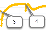
Figure 3: Pressure drop vs iteration. Pressure drop at the final iteration for each mesh is shown in Chart 1. Meshes highlighted are shown in Figure 4. Theoretical pressure drop (blue line) is included for reference. An ultimate answer has not been obtained.
The theoretical pressure drop closely matched the Flow Simulation pressure drop for mesh 6 and 7 at 0.9 and -2.2% error respectively.

Figure 4: 7 details of meshes produced during the 16 hour run. Refer to mesh 1 for location of each detail the scale is the same for all except 7-closeup. See figure 3 for the iterations where each mesh is used.
Mesh 1 is the original user created mesh that started the refinement process. Initially all cells are too coarse and all get divided (meshes 1 and 2 figure 4). Mesh 3 is the first to present cells at the flow centerline that have reached convergence and remained undivided in all the remaining meshes. In each further mesh, cells near the boundary layer reach convergence, but the cells at the wall do not reach convergence and continue to divide. It is expected that if further meshes could be computed, they would have further divided cells at the wall.
Boundary conditions.

Figure 5: Flow velocity probe locations. Inlet and A are 1 pipe diameter (0.01905 m or 0.75″) apart. Same for A to B, B to C and C to D. The red box is the location of the mesh details shown in figure 4.
The velocity of the flow is measured at the inlet, four locations each separated by 1 pipe diameter, and the outlet. At each location, the velocity is measured from the outer edge to the flow centerline.

Figure 6: Velocity distributions, wall to the left, flow centerline to the right. All results are from iteration 763 (the final iteration of mesh 7, the final mesh used).
Velocity profiles for the inlet, locations A to D and the outlet. Results are from the final iteration of the final mesh. The inlet condition is set as “fully developed”, but the flow still takes some distance to develop. See figure 6:
- Inlet – partially developed velocity distribution – this is the Flow Simulation built in fully developed flow distribution.
- Location A – usable but not great – this is one pipe diameter away from the inlet. Differences between the outlet and this location are most apparent at the center line.
- Location B, C, D and outlet – these are good, but changes can be seen compared to the outlet even for location D.
By one pipe diameter, a usable boundary layer has developed. By two diameters, it is close enough to the outlet profile to not matter. This distance to develop a boundary layer in the pipe makes it more unlikely that the Flow Simulation result can exactly match the theoretical value without redesigning the experiment to account for this.
It is up to the user to determine if models being studied need to be modified to allow extra length for boundary layers to develop before areas of interest.
Computational Limits
This validation study is a very simple shape – a small portion of a straight pipe further simplified through symmetry. Unlike the heat transfer validation case, this pressure drop study is very slow to converge with no final pressure drop obtained. The final meshes did produce impressive results within 0.9 and 2.2% of the theoretical answer. However the computational resources used are extreme. A more complex real world problem would have much more detail and complexity, requiring a much coarser mesh. Taking the results as far as mesh 4 and mesh 5 would be more likely. At these meshes the error rate is in the 12 and 10% range for this problem.
For real problems where Flow Simulation would be used no theoretical comparisons are available. Further, each problem has its own convergence pattern (compare with the convergence plots for the flat plate and the elbows on this page). For these real pressure drop problems the operator will be faced with results that are not converged, and with no theoretical results to provide a bounds on the amount of error. This seems grim, but very useful results can be obtained using relative instead of absolute pressure drop information. Please refer to the elbow study on this page for our way to get robust results.

Product Design by Comparative Pressure Drop
Product Design by Comparative Pressure Drop
PVE-11652 LRB / CBM – May 17 2017
The validation study on flow in a straight pipe ran into difficulty determining the ultimate pressure drop. Each time the mesh was further refined, a new pressure drop was calculated. A final answer was not calculated even for extreme mesh sizes run over an entire weekend. An approximate answer was possible, but without assurances that it was the final answer. How can this CFD tool be useful?
When the ultimate pressure drop is not the goal, a way forward is available. In this exercise, two similar designs for 180° pipe elbows are compared. We do not need the absolute pressure drop. The goal is to find which has the lower pressure drop. How easy is it to get this result? And finally, can this method be used on more complex objects?

Figure 1: Two 180° flow elbows to be compared. Section view. Which has the lower pressure drop? “U” configuration on left, “LR” for larger radius on right.
Like the previous validation sets, an initial very coarse mesh is used. Flow Simulation is set to refine the mesh where required until all areas converge and no further mesh refinement is required. Inlet velocity to both elbows is 1 m/s water at 293.2 K and 1 atmosphere. Half symmetry on the XZ plane isused to reduce the complexity of the model. Flow Simulation was set to monitor the pressure drop across both elbows, and compute the ratio of the pressure drop in the “U” design to that of the “LR” design (LR/U – numbers greater than 1 indicate that the pressure drop is larger in the LR case).
The inside flow passage diameter for both elbows is 0.019 m (0.75″). Both have a leg to leg spacing of 0.0508 m (2″). The bend radius of the U design is 0.0254 m (1″) with a 0.0369 m (1.45″) inlet section and a 0.1511 m (5.95″) outlet straight pipe section to allow flow to develop before and after the elbow. The LR design has a larger bend radius of 0.0285 m (1.125″) and the inlet and outlets are reduced in length to allow for a 0.019 m (0.75″) long flow offset section.
The initial coarse mesh (fig 1) was solved by Flow Simulation over 240 steps over which time the pressure drop ratio reached a rough convergence. As the convergence was too rough to allow automatic refinement, the iteration for refinement was chosen by the operator during the run. Total run time was 3 hours on a medium power computer: i7 6600U CPU @ 2.6-2.81 GHz (2 physical cores, 4 hyper threaded cores), 16 GB ram (14 GB used).

Figure 2: Initial mesh used. Results are not expected to be useful, but the program uses the results from each mesh size to determine where more refinement is required in the next mesh.

Figure 3: Final mesh (#6) detail for “LR” elbow. many areas of the mesh have reached convergence and their final mesh size, areas of turbulence and the boundary layer are still being refined (darkest areas with the smallest cells).

Figure 4: Midplane velocity profiles for the final mesh size. The flow pattern is not simple, and the “LR” elbow (right) has a more complex pattern than the “U” elbow (left).

Figure 5: Complex flow patterns around the elbows. This is from the final mesh size (mesh 6).

Figure 6: Pressure drop for the “U” elbow (green) and “LR” (red). The pressure drop graphs did not reach convergence before the run was stopped. However, the results are still useful. Refinement points are shown as “*”.

Figure 7: The ratio of the two pressure drops from figure 6. Useful and consistent information emerges that can be used to compare the two elbows. The highlighted areas are the areas used for the averages.
From Figure 7 – mesh densities for 1 and 2 are too coarse to accurately capture the complexity of the flow going through the elbows and should be ignored. Meshes densities 3 and 4 are typical of what is attainable in a practical flow problem. These results are obtained after 6 minutes (362 s). Mesh sizes 5 and 6 are probably not attainable in real world problems more complicated than this simple flow example. Taking the results from meshes 3 and 4, the “LR” elbow is expected to have a pressure drop about 7.6 to 7.8% higher than the “U” shaped elbow.
Although the pressure drop has not converged, it can clearly be seen that the “U” shaped elbow has a lower pressure loss. This calculation was easily within the reach of the medium powered computer used.
